Simulate species distribution data for RAP

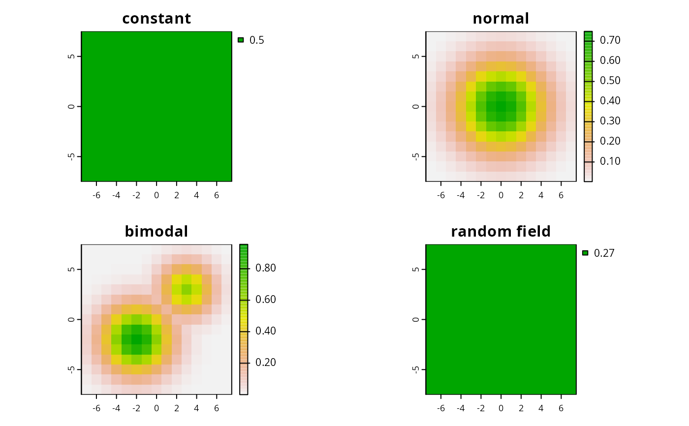
This function simulates species distributions for RAP.

sim.species(x, ...)

# S3 method for SpatRaster
sim.species(x, n = 1, model = "normal", ...)

# S3 method for SpatialPolygons
sim.species(x, res, n = 1, model = "normal", ...)

# S3 method for sf
sim.species(x, res, n = 1, model = "normal", ...)

Arguments

x

terra::rast() or sf::st_sf() object delineating the spatial extent for the study area.

...

not used.

n

integer number of species. Defaults to 1.

model

character or numeric for simulating data. If a character value is supplied, then the following values can can be used to simulate species distributions with particular characteristics: "uniform", "normal", and "bimodal". If a numeric value is supplied, then this is used to simulate species distributions using a Gaussian random field, where the numeric value is treated as the scale parameter. Defaults to "normal".

res

numeric resolution to simulate distributions. Only needed when sf::st_sf() are supplied.

Value

terra::rast() with layers for each species.

Examples

# \dontrun{
# make polygons
sim_pus <- sim.pus(225L)

# simulate 1 uniform species distribution using SpatRaster
s1 <- sim.species(blank.raster(sim_pus, 1), n = 1, model = "uniform")

# simulate 1 uniform species distribution based on sf
s2 <- sim.species(sim_pus, res = 1, n = 1, model = "uniform")

# simulate 1 normal species distributions
s3 <- sim.species(sim_pus, res = 1, n = 1, model = "normal")

# simulate 1 bimodal species distribution
s4 <- sim.species(sim_pus, res = 1, n = 1, model = "bimodal")

# simulate 1 species distribution using a random field
s5 <- sim.species(sim_pus, res = 1, n = 1, model = 0.2)

# plot simulations
par(mfrow = c(2,2))
plot(s2, main = "constant")
plot(s3, main = "normal")
plot(s4, main = "bimodal")
plot(s5, main = "random field")

# }